Monday, July 16, 2012
Lightning
Lightning captured at 7,207 images per second from ZT Research on Vimeo.
A downward lightning negative ground flash captured at 7,207 images per second. A negative stepped leader emerges from the cloud and connects with the ground forming a return stroke.
Friday, July 13, 2012
Auroral on July 14
The night of July 14th, Auroral activity will be high. Depending on weather it should be visible low on the horizon everywhere down to Boston latitude.
This is due to a significant event located on the sun --facing earth-- took place on July 12.
Link to the map
Link to the map
Thursday, July 12, 2012
my long article on physics 13
The university where I work, publishes a journal for undergraduate students titled "Phyics 13". You can google it along with the university of waterloo to find their webpage.
They asked me to write an overview on the recent experiment on the Majorana Quasiparticle recently discovered in Condensed matter physics. Along the way to write it I realized this is much beter if I can glue together a more extensive review on the prediction, the particle physics and astrophysics attempts, as well as a good and simple explanation of its final discovery on a proximity superconducting nanowire of semiconductor. Previously in this blog I wrote about this important discovery.
My extensive review --compared to regular articles-- was published in the latest journal issue. Unfortunately you cannot see the latest issue on their webpage but with a negligible fee for registration to the physics department of the university you can buy a hard copy of it.
The article is now on the Spring 2012 issue on the Young Researcher Corner section, which is now of course a few pages long with many colorful picture! You can read all the previous issues on their website, though.
Wednesday, July 11, 2012
Errors scientists may make
To an extent, I realized that some fields of science proceed only by consensus instead of scientific arguments. This is unfortunately true.
Consensus usually gets things wrong in science because whatever everyone may agree upon may turn out to be completely wrong. There are many examples such as the ultraviolet catastrophe, or more recently black hole information paradox. Things get even worse in research fields for which there are not much experiments available, e.g. quantum gravity. There are many versions of quantum gravity but usually any discovery using one version of the theory may generate strong reactions from people working on the other versions of the theory and most of the times the discussions between the scientists go out of any scientific measure. This sometimes makes a discovery not even be published, which is obviously unfair. Sometimes peers take an illegitimate step to engineer a wall in front of papers written in a version of quantum gravity for the purpose of drying the field out. Arguments in the peer reports turn instead of being "no-physical-evidence-for-the-discovery" to "correct-calculation-based-on-wrong-theory"! Even the peers may advise the authors to change their field and no longer burn themselves in the field.
Science is often presented as an objective pursuit, but the modern academia is unhealthy and cannot afford all novel ideas.
And this is only my thought.
Monday, July 09, 2012
Higgs, and me on a train


In canada we actually benefit from the free strong wifi inside a VIA train and now I am sitting on train and writing this short note.
Sean Carroll seems to be writing a new book on the Higgs boson at the End of the Universe: (a pre-existence review):
Article
Public needs that specially that it is difficult to find an article with less journalistic flavour on Higgs these days.
P.S. Picture above: the three first theorists who predicted the Englert-Higgs-Brout particle, aka. Higgs particle, respectively from left to right.
Friday, July 06, 2012
Quantum mechanics with taste of cabbage roll
Yesterday our institute hosted Helen Fay Dowker. She gave a talk at our traditional thursday lunch meetings and the title was something like the path integral interpretation of quantum mechanics.
Fay gave an introduction about Dirac's 1932 paper that the lagrangian approach to classical mechanics was probably more fundamental than the hamiltonian approach because the former is relativistically invariant whereas the latter is "essentially nonrelativistic." This is because in the definition of hamiltonian time is an exceptional dimension and the evolution occurs in that dimension. This breaks the equality between time and space that general relativity is based on.
In a path integral we sum over histories from which the physical world is described directly in terms of events in spacetime. The path integral approach, however,has been championed in more recent times by Jim Hartle in a probabilistic nature and by Raphael Sorkin in non-probabilistic nature.
 It was almost half past since I put the last piece of the cabbage rolls in my mouth that Tony Leggett asked whether Sorkin's approach with its zero measure can potentially give rise to Yang's experiment... . I remembered a few years ago when I was at the Perimeter Institute in a talk Raphael gave about his causal set I asked this question in a very shaky way with lots of fears and he gave answers but the end of the story as far as I remember was that he didn't know, but he has thought about that.
This path integral talk would have been tasted better with noodles, of course!
And that is my memo.
Fay gave an introduction about Dirac's 1932 paper that the lagrangian approach to classical mechanics was probably more fundamental than the hamiltonian approach because the former is relativistically invariant whereas the latter is "essentially nonrelativistic." This is because in the definition of hamiltonian time is an exceptional dimension and the evolution occurs in that dimension. This breaks the equality between time and space that general relativity is based on.
In a path integral we sum over histories from which the physical world is described directly in terms of events in spacetime. The path integral approach, however,has been championed in more recent times by Jim Hartle in a probabilistic nature and by Raphael Sorkin in non-probabilistic nature.

This path integral talk would have been tasted better with noodles, of course!
And that is my memo.
Wednesday, June 20, 2012
Quantum computer for high school students

Recently some high school students contacted me for an interview. This motivated me to write the following short post on what does it mean to do a quantum computation.
1) What is the difference between a quantum and classical computer?
A)
Let me give you an example, if you want to sum 23 and 45 using classic computers, these numbers are first to be converted from decimal format to binary (0 and 1): 23 in decimal =10111 in binary, and 45=101101.
These two binaries must be written in left to right column order and they are linked together using a "summation" operator applied at each column. So we need 6 summation operators to work on the inputs. In quantum computers however, each number is represented by an angle and the summation of two number (no matter how large they are) needs at least one summation operator (that adds the angles).
What is the angle?
In quantum bits (qubit), we can have both states of 0 and 1 at the same time. So the state of a qubit can be 0 or 1 or a superposition of the two: a*(state 0)+b(state 1), where a and b are not independent coefficients, they are linked together by the relation a^2+b^2=1, so we have only one of them as an independent variable. You can assume state 0 is linka vector along the axis x and the state y is a vector along the axis y. Given the two states we can make any combination of the two vectors as a vector from the origin toward any direction in the xy plane. The angle between the vector and the axis x is related to the coefficient a (in fact the tangent of the angle is tan(theta)=b/a=sqrt(1-a^2)/a.)
This angle can be discretized in units (a unit is a small angle we can distinguish depending on the noise etc. in the system) and we can calibrate each unit to represent one in the decimal numbers.
This way adding two numbers means adding two angles. For this we need one summation operator and this saves a lot of resources in the computation. Similarly very complicated calculations can be achieved using smaller number computer resources compared to classical computers.
2) What are the main restrictions in making quantum computers, and how soon can we expect quantum computers to be put in use, and perhaps put on the market?
There are many different quantum computer version from ion trap to superconducting qubits and quantum optic. The smallest and most portable one is superconducting qubits, however they need to operate in low temperature (as low as 1 kelvin or lower). If we can achieve higher temperature less noisy system that may make a way into market.
Search for D-wave quantum computer to read about a 10million machine that was made recently.
3) How much faster is a quantum computer than an 8-bit computer?
People say exponentially faster. For the example I said earlier on the summation if each summation operator needs 0.1 second to take place, 6 of them in a row for summing 23 and 45 needs at least 0.6 second in classical computers, however only one of the operators is required in quantum computers and therefor 6 times faster (0.1 second). You can assume for large numbers the different becomes more pronounced. For instance a large factorial operator that takes years to compute on classical computers can be calculated in a few second.
To read more ... there are plenty of good references and book online. A few of them are:
http://www.scottaaronson.com/writings/highschool.html
http://michaelnielsen.org/blog/quantum-computing-for-everyone/
Also at our institute you can find very interesting programs to attend
and learn more about qubits.
Wednesday, May 30, 2012
Done with the lectures
At the end of the lectures the grad students saw the formulae I derived in the course fit onto recent experimental data!
and now? it is time for designing assignment in grad scales...
Lecture 3.pdf
Lecture 4.pdf
Comparing theory with experiments
More about te course available at the course homepage.
and now? it is time for designing assignment in grad scales...
Lecture 3.pdf
Lecture 4.pdf
Comparing theory with experiments
More about te course available at the course homepage.
Friday, May 25, 2012
2nd lecture on nanowire theory at IQC
2nd lecture was joyful and full of my simple derivations.
I talked about two fluid model of Gorter and Casimir and derived many interesting things including the temperature dependence of penetration depth. Then derived deviations of penetration depth from that of London in non-local type II pure superconductors. After that I derived penetration depth for thin film for the two cases of parallel and perpendicular magnetic fields. A little touch on Ginzburg-Landau theory and derived their equation, then talked about the physical meaning of parameters.
Students (and postdocs) were happy and had plenty of high quality questions. They are very sharp! Looking forward for the 3rd lecture on Monday!
Lecture note 2.pdf
Wednesday, May 23, 2012
First lecture at IQC
The first lecture on nanowire theory at IQC went unexpectedly well today!
The title of the course is rather long: "Superconducting and Semiconducting nanowires and Low Energy Physics." This is a module out of 10 modules for a quantum information theory course accessible to graduate students of physics, computer science, and electrical engineering. The list of other modules are here.
In the first lecture, I discussed two-fluid model, London equations, and Boltzmann equation and using them I derived coherence length and the magnetic penetration depth with and without non-locality effect, and in pure and dirty bulk superconductors. Most of the derivations were made by myself in a radically simple way with (or perhaps without) minimal confusions for students.
I am looking forward to the second lecture, which should be a lot of fun!
Lecture note 1.pdf
Thursday, April 26, 2012
Another experiments on Majorana quasiparticles this week, but...
Majorana, the third!
Last week, two groups reported the discovery of a pair of Majorana quasiparticles at the end of a semiconductor wire.
Their probe was the creation of zero energy level in the two ends of the wire. Applying bias current through the wire and measuring conductance of the wire in the lack and presence of magnetic field indicates: whenever the field above a limit is applied on the wire (perpendicular to internal spin-orbit moment), a "strange" zero energy levels appears. This energy level is firmly stuck on the zero energy (doesn't want to split or shift from zero a bit in stronger fields!) This is similar to what expected from Majorana quasiparticles.
Browsing arXiv shows one other experiment has been completed in similar setups (submitted 3 days before Kouwenhoven submit their initial work) in which a signature other than the zero energy level of these particles is experimented.
In this work, on the same setup as used now they applied an rf voltage on the wire and measured the IV plot. The Shappiro steps was observed. These steps were already known from the Josephson junction studies. When rf voltage applies on a Josephson junction the voltage causes phase difference in the junction to oscillate. When this is considered in the supercurrent-phase relation (i.e. I=sin(phase)), gives rise to some phase lock-ins at harmonics of the rf frequency. The amplitude of the beatings is sensitive to the power of the rf voltage. In other words, the average voltage jumps from one value to another by the increase of bas current through the wire.
The precise fact about these steps is that the size of the voltage steps is inversely proportional to the charge of carrier particles. If the carrier is of charge e' the step size is proportional to 1/e'. For instance, in a Josephson junction that the carriers are cooper pairs the step sizes are proportional to 1/(2*e).
Rokhinson, Liu and Furdyna in this paper show similar effect (instead of a Josephson junction, now) on the InSn nanowire in the setup used for observation of Majorana. Interestingly they observed without magnetic field the voltage steps are proportional to 1/(2*e). When they apply 2.7T along the wire they start to observe the size of the steps is doubled, which means in the new regime the carriers have the charge e instead of 2*e. Below, you see the doubling of the size of steps:
Although they found an interesting phenomenon, but in their supplementary material their fitting Bessel function seems not to be perfectly approved experimentally!
Nonetheless, The only concern is that the magnetic field required to create the Majororana in InSb is 100mT applied along the wire. In this experiment, they do not see the effect even at 20 times larger field and only started to observe the effective e-charge carrier at B~2.7T. Note that in 1T the zero bias voltage starts to split so it is likely the Majorna quasiparticles are mixed up with something else of the type of Kondo levels (look at the plot of "Fig.2" in here.)
Is this really due to Majorana quasiparticle? Maybe...
Last week, two groups reported the discovery of a pair of Majorana quasiparticles at the end of a semiconductor wire.
Their probe was the creation of zero energy level in the two ends of the wire. Applying bias current through the wire and measuring conductance of the wire in the lack and presence of magnetic field indicates: whenever the field above a limit is applied on the wire (perpendicular to internal spin-orbit moment), a "strange" zero energy levels appears. This energy level is firmly stuck on the zero energy (doesn't want to split or shift from zero a bit in stronger fields!) This is similar to what expected from Majorana quasiparticles.
Browsing arXiv shows one other experiment has been completed in similar setups (submitted 3 days before Kouwenhoven submit their initial work) in which a signature other than the zero energy level of these particles is experimented.
Here it is:
"Observation of the fractional ac Josephson effect: the signature of Majorana particles", by Leonid P. Rokhinson, Xinyu Liu, and Jacek K. Furdyna, arXiv:1204.4212
In this work, on the same setup as used now they applied an rf voltage on the wire and measured the IV plot. The Shappiro steps was observed. These steps were already known from the Josephson junction studies. When rf voltage applies on a Josephson junction the voltage causes phase difference in the junction to oscillate. When this is considered in the supercurrent-phase relation (i.e. I=sin(phase)), gives rise to some phase lock-ins at harmonics of the rf frequency. The amplitude of the beatings is sensitive to the power of the rf voltage. In other words, the average voltage jumps from one value to another by the increase of bas current through the wire.
The precise fact about these steps is that the size of the voltage steps is inversely proportional to the charge of carrier particles. If the carrier is of charge e' the step size is proportional to 1/e'. For instance, in a Josephson junction that the carriers are cooper pairs the step sizes are proportional to 1/(2*e).
Rokhinson, Liu and Furdyna in this paper show similar effect (instead of a Josephson junction, now) on the InSn nanowire in the setup used for observation of Majorana. Interestingly they observed without magnetic field the voltage steps are proportional to 1/(2*e). When they apply 2.7T along the wire they start to observe the size of the steps is doubled, which means in the new regime the carriers have the charge e instead of 2*e. Below, you see the doubling of the size of steps:
 |
| Fig1. The y-axis is the average voltage measured in the wire. Left graph shows in small magnetic field the steps are still proportional to the cooper pair charge, however when the wire is bring to higher magnetic field in which Majorana should appear the size of the steps is doubled which means the carrier of charge e are coherent at zero energy level. These new carrier are perhaps Majorana quasiparticles. |
Although they found an interesting phenomenon, but in their supplementary material their fitting Bessel function seems not to be perfectly approved experimentally!
Nonetheless, The only concern is that the magnetic field required to create the Majororana in InSb is 100mT applied along the wire. In this experiment, they do not see the effect even at 20 times larger field and only started to observe the effective e-charge carrier at B~2.7T. Note that in 1T the zero bias voltage starts to split so it is likely the Majorna quasiparticles are mixed up with something else of the type of Kondo levels (look at the plot of "Fig.2" in here.)
Is this really due to Majorana quasiparticle? Maybe...
Thursday, April 19, 2012
"Majorana" made two times last week!
Last week, two different groups, one at Delft and the other from Sweden, France, and China, reported observation of the "Majorana quasiparticle" in condensed matter.
(1) V Mourik, K Zuo, S M Frolov, S R Plissard, E P A M Bakkers, and L P Kouwenhoven, "Signatures of Majorana fermions in hybrid superconductor-semiconductor nanowire devices"
http://arxiv.org/abs/1204.2792
Science DOI: 10.1126/science.1222360
Downloadable at Delft group in Science format: here
(2) M. T. Deng, C. L. Yu, G. Y. Huang, M. Larsson, P. Caroff, H. Q. Xu, "Observation of Majorana Fermions in a Nb-InSb Nanowire-Nb Hybrid Quantum Device", http://arxiv.org/abs/1204.4130v1
(Appeared today and apparently will be published in Nature Physics)
Here I discuss the underlying physics of the phenomenon and the differences between the two experiments.
A semiconductor wire with high Lande g-factor shows splitting of the well-known energy-momentum parabola into two shifted parabolas one to the left and one to the right for spin up and spin down electrons (figure below). In magnetic field these two parabola are smeared and a parabola becomes nested inside a double-minima parabola (black lines in the figure below.) The gap between the two black parabola is called Zeeman gap. Note also the point where blue and red curves collide are usually set to be the chemical potential.
If s-wave superconductivity is proximated to this wire, an induced gap appears that tries to couple two "almost" parallel spins. Note that for s-wave superconductor in trivial phase (regular sense) the pairing occurs between spin up and down. In fact, the proximity of regular s-wave superconductor to a material with large spin-orbit interaction makes it possible to induce p-wave superconductor!
If the induced superconductivity gap is too large (larger than the Zeeman gap) a regular p-wave superconductor must appear, but in the opposite case a two-fold degenerate ground state at zero energy appears that is topologically non-trivial, the so-called "the Majorana fermions."
Both of these groups made similar devices with minor differences. In (1) a Gold reservoir plate placed next to a NbTiN superconductor reservoir plate, in (2) both plates are NbTi. Between the two there is almost 200nm gap, under which there are some gate voltages. An InSb semiconductor was placed on the top of the two reservoirs and the gap between. The gate voltage (shown in above figure in green line) can make a tunnel junction in the nanowire due to the electrical repulsion (large electric potential barrier).
Now, both of the groups apply a magnetic field along the wire perpendicular to the spin orbit internal magnetic field. However group (1) applies it parallel with the wire first and then applies it in any orientation, the group (2) applies it only perpendicular to the substrate and the wire. This turns on the Zeeman gap in both cases. If the Zeeman gap be smaller than the superconducting gap a regular superconductor is made, but if is stronger and beats the superconducting gap the "Majorana" fermions starts to show up from. Given the induced superconducting gap in the wire between the two plates (before the tunnel gate in the superconducting side) is 0.25meV, one can finds the minimum magnetic field required for the Majorana fermions to appear ---"(superconducting gap)=(1/2)(Bohr magneton)(g-factor)(magnetic field)." The required magnetic field is B>150mT.
In group (1) experiment the magnetic field is exposed to any orientations. They saw whenever it is perpendicular to the spin-orbit internal field a zero energy level appears (from which the conduction of cooper pairs becomes possible). This zero energy level was checked to see if it has a different nature such as Kondo effect or Andreev reflection. These two latter phenomena are ruled out because the zero energy levels they detect is insensitive to the external magnetic field. So the only scenario left that describes this insensitivity is that the Majorana fermions are located at the zero energy levels from which the tunneling is occurring.
In following figure, the neat result of group (1) is shown in top where the result of the group (2) is below it:

As you see both works are similar, both of them saw
1- the induced superconducting gap to be 0.25meV,
2- chemical potential is set to zero, and
3- the semiconductor in both works are InSb.
Rough calculation shows that the Majorana fermions should be seen in about 150mT. In the work (1) they saw it there, but in the work (2) they see zero bias peak in 10 times larger magnetic field (about 1T).
What is puzzling is that why there is this difference in the magnetic field threshold of observing the zero bias peak? (In group (1) the threshold is 150mT in group (2) it is above 1T.)
Indeed the puzzle is already solved at the end of the work (1).
Group (1) produces results of the conductance by changing the angle of magnetic field and the nanowire and the substrate. They first change the magnetic field orientation parallel to the substrate. Note they define the angle to be between field and wire. This means magnetic field when is in 0 and pi degrees with the wire, it is perpendicular to the spin orbit magnetic and only in this case Majurana fermions appears (because only when the external field is perpendicular to the spin-orbit internal magnetic field spinless fermions can pair up via superconductivity and produce a funny quasiparticle called "the Majurana fermion.") In the following figure, the top graph shows that zero voltage peak only exists at the angle 0 and pi.
Below it, they show the result where the external magnetic field is in a plane perpendicular to the spin-orbit magnetic field. In this case, the angle between the spin orbit and external magnetic fields is always 90 degrees and Majorana fermions is seen at any angle, so as you see the zero bias peak is seen at any angle.
However, in work (2) the magnetic field is only perpendicular to the substrate, which is only one case among many from the lower graph, shown here by the yellow dashed line. This angle point is no convenient for this experiment due to the presence of many conduction levels. In fact this part of the graph is very "dirty" and crowded with other levels that makes it unsuitable for measurement. This is the main reason why they had to apply this huge (and problematic) magnetic field to push away all the Kondo and Andreev zero energy states (thanks to their magnetic field dependency) such that only Majurana fermions are left intact at zero energy.
In my point of view, although both works appear at the same time (the work of group (1) on March 23, 2012 and the work of group (2) on March 27, 2012) and although the quality of the work (1) is more convincing than (2), but both of these two works should be considered as the first signature of the artificial "Majorana" fermions.
For more information about theory read the paper by Lutchyn as well as Oreg in the list of references in the papers.
(1) V Mourik, K Zuo, S M Frolov, S R Plissard, E P A M Bakkers, and L P Kouwenhoven, "Signatures of Majorana fermions in hybrid superconductor-semiconductor nanowire devices"
http://arxiv.org/abs/1204.2792
Science DOI: 10.1126/science.1222360
Downloadable at Delft group in Science format: here
(2) M. T. Deng, C. L. Yu, G. Y. Huang, M. Larsson, P. Caroff, H. Q. Xu, "Observation of Majorana Fermions in a Nb-InSb Nanowire-Nb Hybrid Quantum Device", http://arxiv.org/abs/1204.4130v1
(Appeared today and apparently will be published in Nature Physics)
Here I discuss the underlying physics of the phenomenon and the differences between the two experiments.
A semiconductor wire with high Lande g-factor shows splitting of the well-known energy-momentum parabola into two shifted parabolas one to the left and one to the right for spin up and spin down electrons (figure below). In magnetic field these two parabola are smeared and a parabola becomes nested inside a double-minima parabola (black lines in the figure below.) The gap between the two black parabola is called Zeeman gap. Note also the point where blue and red curves collide are usually set to be the chemical potential.
 |
| Fig1: (A): Top: A part of the nanowire on the superconductor hosts two Majorana fermions at the red stars. Below: Red and Blue are spin-orbit states in the lack of external magnetic field and the black parabola are those in the presence of magnetic field. (B) Actual circuit of group (1), the green shows where the tunneling gate is placed between Superconductor S and the normal metal N reservoirs. |
If s-wave superconductivity is proximated to this wire, an induced gap appears that tries to couple two "almost" parallel spins. Note that for s-wave superconductor in trivial phase (regular sense) the pairing occurs between spin up and down. In fact, the proximity of regular s-wave superconductor to a material with large spin-orbit interaction makes it possible to induce p-wave superconductor!
If the induced superconductivity gap is too large (larger than the Zeeman gap) a regular p-wave superconductor must appear, but in the opposite case a two-fold degenerate ground state at zero energy appears that is topologically non-trivial, the so-called "the Majorana fermions."
Both of these groups made similar devices with minor differences. In (1) a Gold reservoir plate placed next to a NbTiN superconductor reservoir plate, in (2) both plates are NbTi. Between the two there is almost 200nm gap, under which there are some gate voltages. An InSb semiconductor was placed on the top of the two reservoirs and the gap between. The gate voltage (shown in above figure in green line) can make a tunnel junction in the nanowire due to the electrical repulsion (large electric potential barrier).
Now, both of the groups apply a magnetic field along the wire perpendicular to the spin orbit internal magnetic field. However group (1) applies it parallel with the wire first and then applies it in any orientation, the group (2) applies it only perpendicular to the substrate and the wire. This turns on the Zeeman gap in both cases. If the Zeeman gap be smaller than the superconducting gap a regular superconductor is made, but if is stronger and beats the superconducting gap the "Majorana" fermions starts to show up from. Given the induced superconducting gap in the wire between the two plates (before the tunnel gate in the superconducting side) is 0.25meV, one can finds the minimum magnetic field required for the Majorana fermions to appear ---"(superconducting gap)=(1/2)(Bohr magneton)(g-factor)(magnetic field)." The required magnetic field is B>150mT.
In group (1) experiment the magnetic field is exposed to any orientations. They saw whenever it is perpendicular to the spin-orbit internal field a zero energy level appears (from which the conduction of cooper pairs becomes possible). This zero energy level was checked to see if it has a different nature such as Kondo effect or Andreev reflection. These two latter phenomena are ruled out because the zero energy levels they detect is insensitive to the external magnetic field. So the only scenario left that describes this insensitivity is that the Majorana fermions are located at the zero energy levels from which the tunneling is occurring.
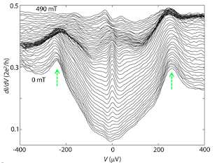
In following figure, the neat result of group (1) is shown in top where the result of the group (2) is below it:

Fig.2: Result of Group (1): Zero voltage conductance indicates Majorana

Fig.3: Result of group (2): The zero voltage conductance in 10 times larger magnetic field indicates Majorana
1- the induced superconducting gap to be 0.25meV,
2- chemical potential is set to zero, and
3- the semiconductor in both works are InSb.
Rough calculation shows that the Majorana fermions should be seen in about 150mT. In the work (1) they saw it there, but in the work (2) they see zero bias peak in 10 times larger magnetic field (about 1T).
What is puzzling is that why there is this difference in the magnetic field threshold of observing the zero bias peak? (In group (1) the threshold is 150mT in group (2) it is above 1T.)
Indeed the puzzle is already solved at the end of the work (1).
Group (1) produces results of the conductance by changing the angle of magnetic field and the nanowire and the substrate. They first change the magnetic field orientation parallel to the substrate. Note they define the angle to be between field and wire. This means magnetic field when is in 0 and pi degrees with the wire, it is perpendicular to the spin orbit magnetic and only in this case Majurana fermions appears (because only when the external field is perpendicular to the spin-orbit internal magnetic field spinless fermions can pair up via superconductivity and produce a funny quasiparticle called "the Majurana fermion.") In the following figure, the top graph shows that zero voltage peak only exists at the angle 0 and pi.
Below it, they show the result where the external magnetic field is in a plane perpendicular to the spin-orbit magnetic field. In this case, the angle between the spin orbit and external magnetic fields is always 90 degrees and Majorana fermions is seen at any angle, so as you see the zero bias peak is seen at any angle.
 |
| Fig.4: From group (1): Seen here the reaction of zero voltage conductance to the external magnetic field orientation. Angle defined between the field and the wire. In (A) zero energy state conductance is seen at angle 0, pi and 2 pi because only at these angles the external magnetic field is perpendicular to the internal spin orbit magnetic field. In (B) the external field takes angles in the plane perpendicular to the spin orbit field and thus the Majorana is seen at all angles. |
However, in work (2) the magnetic field is only perpendicular to the substrate, which is only one case among many from the lower graph, shown here by the yellow dashed line. This angle point is no convenient for this experiment due to the presence of many conduction levels. In fact this part of the graph is very "dirty" and crowded with other levels that makes it unsuitable for measurement. This is the main reason why they had to apply this huge (and problematic) magnetic field to push away all the Kondo and Andreev zero energy states (thanks to their magnetic field dependency) such that only Majurana fermions are left intact at zero energy.
 |
| Fig.5: Shown in dashed line the single angle at which group (2) did their experiment. They chose a dirty part of the spectrum to see Majorana. |
In my point of view, although both works appear at the same time (the work of group (1) on March 23, 2012 and the work of group (2) on March 27, 2012) and although the quality of the work (1) is more convincing than (2), but both of these two works should be considered as the first signature of the artificial "Majorana" fermions.
For more information about theory read the paper by Lutchyn as well as Oreg in the list of references in the papers.
Wednesday, April 18, 2012
Quantum Noise and Measurement in Engineered Electronic Systems
Quantum Noise and Measurement in Engineered Electronic Systems
Here
International Workshop – 8 - 12 October 2012
Organisation:
Katrin Lantsch (Max-Planck-Institut für Physik komplexer Systeme Dresden, Germany)
The list of invited speakers includes:
T. Brandes (Berlin, Germany), M. Büttiker (Geneva, Switzerland), A. Clerk (Montreal, Canada), L. DiCarlo (Delft, The Netherlands), K. Ensslin (Zürich, Switzerland), D. Esteve (Gif-sur-Yvette, France), Y. Gefen (Rehovot, Israel), S. Girvin(New Haven, USA), D.C. Glattli (Gif-sur-Yvette, France), M. Heiblum (Rehovot, Israel), T. Kippenberg (Lausanne, Switzerland), J. König (Duisburg, Germany), T. Kontos (Paris, France), G.B. Lesovik (Moscow, Russia), L. Levitov(Cambridge, USA), F. Marquardt (Erlangen, Germany), T. Martin (Marseille, France), K. Mølmer (Aarhus, Denmark),J. Pekola (Aalto, Finland), B. Reulet (Sherbrooke, Canada), R. Schoelkopf (New Haven, USA), G. Schön (Karlsruhe, Germany), C. Schönenberger (Basel, Switzerland), I. Siddiqi (Berkeley, USA), J. van Ruitenbeek (Leiden, The Netherlands), F. von Oppen (Berlin, Germany), A. Wallraff (Zürich, Switzerland)
Subscribe to:
Posts (Atom)